Lesson 9. Statistical Significance vs Noise
Mission link: Stage 5's go/no-go call is only as good as knowing whether an observed score difference is real; this lesson gives the tools that answer that, building directly on lesson 8's point that a single run's number carries its own noise.
Primary source: Docs: "Define success criteria and build evaluations", Claude Platform Docs
Prerequisites: Lesson 8, Data contamination
Warm-up
- ▢ Why can the same eval, run twice at a nonzero temperature, produce two different aggregate scores without anything being wrong?
Check
Sampling at a nonzero temperature makes generation stochastic, so different completions, and so different per-example scores, are expected across runs. The single-run number is a sample from a distribution, not a fixed fact about the model.
- ▢ What should be logged alongside a reported eval score to make a later comparison meaningful?
Check
The random seed, generation temperature, model and framework versions, eval set version, and, when multiple samples were run, the spread across them, not just their mean.
Know this
A score difference is not automatically a real difference
A new model variant scores 76% against a baseline's 70% on the same eval set. That six-point gap looks like an improvement, but lesson 8 already established that a single run's score carries its own noise from sampling. The question this lesson answers: is a six-point gap bigger than the noise that could produce it by chance alone, or is it exactly the kind of variation two runs of the same model might show against each other?
Sample size sets how much noise to expect
For a pass/fail-style score over N examples, with a true pass rate p, the standard error of the measured proportion is approximately sqrt(p(1−p)/N). A pass rate of 0.70 over 100 examples has a standard error of about sqrt(0.70 × 0.30 / 100) ≈ 0.046, or roughly 4.6 percentage points; a pass rate of 0.76 over the same 100 examples has a standard error of about 4.3 points. A six-point gap between two estimates each carrying roughly four to five points of noise is not obviously larger than what chance alone could produce; more examples would shrink each standard error (it falls with sqrt(N)), tightening the estimate and making a real difference easier to distinguish from noise.
Paired comparison is the sharper tool
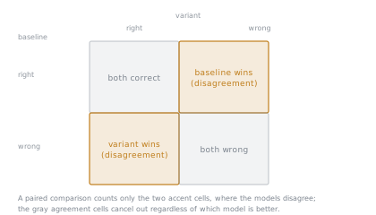
Treating the two scores as independent proportions, the way the estimate above did, throws away information that's actually available: when the same eval examples are run through both the baseline and the new variant, you know not just how many each got right, but which specific examples each got right or wrong. A paired comparison looks at the examples where the two models disagree (one got it right and the other didn't) rather than at the two raw pass rates separately. This cancels out example-level difficulty that affects both models equally, a question every model tends to get right or every model tends to get wrong contributes nothing to whether one model is actually better than the other, and it makes a real difference easier to detect from the same amount of data than comparing two independent proportions would.
What "not yet significant" means for a go/no-go call
A gap that isn't clearly larger than the noise isn't evidence of no difference; it's evidence of not enough information yet to tell. The honest response is either running more examples (shrinking the standard error) or running a proper paired significance test on the disagreements, not treating a numerically larger score as proof of improvement on its own.
Practice
- ▢ A baseline model passes 70 out of 100 eval examples; a new variant passes 76 out of 100. Compute the approximate standard error of each proportion, and say whether the six-point gap looks clearly larger than the combined noise.
Hint
Use sqrt(p(1−p)/N) for each proportion separately, with N = 100.
Check
Baseline: sqrt(0.70 × 0.30 / 100) ≈ 0.046, about 4.6 points. New variant: sqrt(0.76 × 0.24 / 100) ≈ 0.043, about 4.3 points. Each estimate individually carries roughly four to five points of noise, so a six-point gap is not clearly larger than what that combined noise could produce by chance; it's suggestive, not conclusive, on 100 examples alone.
- ▢ Why does using a larger eval set (more examples) make a real score difference easier to distinguish from noise?
Check
The standard error of a proportion falls with sqrt(N), so a larger N shrinks the noise in each estimate. A gap that looked ambiguous against 100 examples' worth of noise can become clearly larger than the noise once measured against, say, 1,000 examples, without the underlying true difference having changed at all.
- ▢ The same 100 eval examples are run through both a baseline and a new variant. Why is looking at which specific examples each model got right or wrong (a paired comparison) more powerful than just comparing the two raw pass rates, 70% and 76%, as independent numbers?
Check
Comparing raw pass rates treats each score as if it came from an unrelated sample, discarding the fact that the same examples were used for both. A paired comparison instead looks at where the two models disagree, canceling out example-level difficulty that affects both equally (a question every model gets right or every model gets wrong says nothing about which model is better), which makes a real difference detectable with less data than an independent-proportions comparison needs.
- ▢ A team observes a score gap between two model variants that turns out not to be clearly larger than the estimated noise. What is the honest conclusion, and what are two ways to get a clearer answer?
Check
The honest conclusion is that there isn't yet enough information to say whether the difference is real, not that there is no difference. Two ways to clarify it: run the eval on more examples, which shrinks each estimate's standard error, or run a proper paired significance test on the specific examples where the two variants disagree, rather than comparing the two raw pass rates as independent numbers.
-
▢ Which claim is true of judging whether an eval score difference is real?
- a) Any positive gap between two scores counts as evidence of improvement, regardless of sample size
- b) A gap should be judged against the noise the sample size could produce by chance, and a paired comparison uses the data more efficiently than treating scores as independent
- c) Statistical significance only matters for task-specific metrics, not LLM-as-judge scores
- d) A larger eval set can never change whether a given gap looks significant
Check
b) Both the noise-versus-sample-size reasoning and the paired-comparison advantage are exactly what this lesson covers. (a) is false: a gap smaller than the estimated noise is not solid evidence, regardless of its sign. (c) is false: the same statistical reasoning applies to any aggregate score, however it was graded. (d) is false: standard error shrinks with sqrt(N), so a larger eval set can turn an ambiguous gap into a clear one.
Real-world reps
- [ ] For a score difference you've observed between two model variants, estimate the standard error of each proportion using this lesson's formula, and check whether the gap is clearly larger than the combined noise.
- [ ] If you have per-example results for both variants on the same eval set, look at the examples where they disagree and count them, as the first step toward a paired comparison.
- [ ] Tomorrow: decide, for an eval you care about, whether its current sample size is large enough to detect the size of improvement that would actually matter for a go/no-go decision.
Going further
Not landing? Reread the primary source at the top, since this lesson compresses it and compression is where understanding leaks. Check the glossary for any term that felt slippery.
If the lesson itself is unclear rather than the material, that is a defect: open an issue.