Lesson 7. Activations, Batch Size and Checkpointing

Mission link: Adapters remove the optimizer cost but not the activation cost, which is why a LoRA run can still run out of memory. This is the part people are surprised by.
Primary source: Paper: "Training Deep Nets with Sublinear Memory Cost", Chen et al., arXiv:1604.06174
Prerequisites: Lesson 6

Warm-up

1. ▢ Bytes per trainable parameter under AdamW, mixed precision?

2. ▢ Bytes per frozen parameter?

3. ▢ Why can't AdamW's moments simply be dropped for transformers?

Know this

Gradients and optimizer state scale with parameter count. Activations scale with batch size and sequence length, and are almost independent of how many parameters are trainable. Freezing the base does not help here at all.

Why activations exist

The backward pass needs each layer's input to compute that layer's gradient. So the forward pass keeps its intermediate results instead of discarding them. Every kept tensor is roughly:

batch_size × sequence_length × hidden_size × bytes_per_element

per tensor, and a transformer block holds a dozen or so of them: after each normalisation, each projection, the attention output, the MLP intermediate at its wider dimension, and so on. Multiply by the number of layers.

A rough working figure for a bf16 transformer block, counting the notable tensors:

activations ≈ n_layers × batch × seq_len × hidden × ~20 bytes

Treat the constant as a starting point to be measured, not a law, because it moves with the attention implementation, the activation function, and whether the framework fuses operations. What matters is the shape of the formula.

The consequences of the shape

Linear in batch size. Double the batch, double activation memory. This is the knob you reach for first, and gradient accumulation (Lesson 4) recovers the effective batch size for free in memory terms.

Linear in sequence length for the stored activations, and quadratic for the attention score matrix, unless you use a memory-efficient attention kernel. Modern implementations such as FlashAttention avoid materialising the full seq_len × seq_len matrix, which removes the quadratic term. If you are still hitting quadratic blow-up on long sequences, the fix is the attention implementation, not the batch size.

Worked, for a 24-layer model with hidden size 2048, batch 4, sequence length 2048:

24 × 4 × 2048 × 2048 × 20 bytes ≈ 8.0 GB

Eight gigabytes of activations, against roughly 2.2 GB of frozen bf16 weights and a few tens of megabytes of adapter state. The activations are now the dominant cost. This is the memory profile of a typical adapter run, and it is the opposite of the full fine-tuning profile from Lesson 6.

Gradient checkpointing

The trade that fixes it: do not store most activations. Store a few, and recompute the rest during the backward pass.

Keep the input to each block (a checkpoint), discard everything inside it, and when the backward pass reaches that block, re-run its forward pass to regenerate what is needed. Storage drops from roughly linear in depth to roughly the square root of it, at the cost of about one extra forward pass, commonly 20 to 40% slower per step.

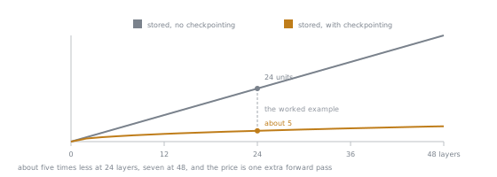
The shape of that trade is why it is close to a default. A straight line and a square root are barely apart at two or three layers, so on a toy model the technique looks pointless; the gap is about five times at the worked example's 24 layers and keeps widening, and the price stays one extra forward pass however deep the model gets.

model.gradient_checkpointing_enable()
model.config.use_cache = False  # incompatible with checkpointing during training

That second line matters. The KV cache exists to speed up autoregressive generation and has no role in training; leaving it enabled alongside checkpointing produces warnings at best and wasted memory at worst.

Gradient checkpointing is close to a default for adapter fine-tuning. It buys back the largest single cost in the profile above, and the slowdown is almost always worth it.

Padding and packing

Every sequence in a batch is padded to the batch's longest member, and padding consumes activation memory while contributing nothing. Two remedies:

• Length grouping. Batch similarly-sized sequences together, so less padding is needed.
• Packing. Concatenate short examples into full-length sequences, eliminating padding almost entirely.

Packing is a real efficiency win on datasets of short examples, and it has a correctness requirement: examples packed together must not attend across their boundaries. Implementations handle this with position resets and boundary-aware attention. If you enable packing, verify that your loss masking survives it: a packed sequence must keep its -100 labels intact, or completion-only loss quietly becomes full-sequence loss.

The order to try things

When a run does not fit, in order of what you give up:

1. Enable gradient checkpointing, which costs time only
2. Reduce per-device batch size and raise gradient accumulation, which costs a little time and changes nothing statistically
3. Reduce sequence length, which changes the task, so check your token-length distribution first
4. Quantise the base model, which is stage 4 and costs some quality
5. Reduce adapter rank, which costs capacity and saves the least of any option here

That last point is worth dwelling on. Rank is the knob people reach for first and it is nearly the least effective, because adapter parameters are a tiny fraction of the total. Halving rank on a 4M-parameter adapter saves 32 MB.

Practice

1. ▢ Which of these scale with trainable parameter count, and which with batch and sequence length: gradients, activations, optimizer moments, frozen weights?

2. ▢ Estimate activation memory for a 32-layer model, hidden size 4096, batch 2, sequence length 4096, bf16.

3. ▢ Your LoRA run runs out of memory. A colleague suggests dropping rank from 64 to 8. Evaluate.

4. ▢ Why must use_cache be disabled when gradient checkpointing is on?

5. ▢ What does gradient checkpointing trade, in both directions?

6. ▢ You enable packing and your model starts producing answers to questions nobody asked. What went wrong?

Real-world reps

• [ ] Run one training step at batch 1, then batch 2, then batch 4, recording peak memory each time. Confirm the relationship is linear.
• [ ] Turn on gradient checkpointing and repeat. Record both the memory saved and the seconds-per-step lost, and decide whether you would take that trade.
• [ ] Tomorrow: measure the token-length distribution of a real dataset with the actual tokenizer. Find the 95th percentile. That, not the maximum, is your sequence length.

Going further

• Paper: "Training Deep Nets with Sublinear Memory Cost", Chen et al., arXiv:1604.06174
• Paper: "FlashAttention: Fast and Memory-Efficient Exact Attention with IO-Awareness", Dao et al., arXiv:2205.14135
• Docs: Methods and tools for efficient training on a single GPU, Hugging Face
• Memory budget: now complete enough to use

Not landing? Reread the primary source at the top, since this lesson compresses it and compression is where understanding leaks. Check the glossary for any term that felt slippery.

If the lesson itself is unclear rather than the material, that is a defect: open an issue.