Lesson 9. Rank, Alpha and Initialisation
Mission link: The mission asks you to justify every hyperparameter from the task. These three are where most people repeat folklore instead.
Primary source: Docs: LoRA, Hugging Face PEFT
Prerequisites: Lesson 8
Warm-up
- ▢ Write the LoRA forward equation.
Check
h = W₀x + (α/r) · BAx, with W₀ frozen and only A and B trainable.
- ▢ Adapter parameter count for one targeted layer?
Check
r × (d_in + d_out). Dominated by the larger dimension.
- ▢ Why does a merged adapter cost nothing at inference?
Check
The update is additive and linear, so it folds into the base weight and leaves an ordinary matrix behind.
Know this
Initialisation, and why it is not arbitrary
A is initialised randomly, either Gaussian or Kaiming-uniform. B is initialised to exactly zero.
Therefore BA = 0 at step zero, so ΔW = 0, so the adapted model is bit-for-bit the base model before the first update. This is a deliberate and important property:
- Training starts from a known-good model rather than a perturbed one.
- There is no initial shock to pretrained behaviour, so no early damage to undo.
- Any degradation you observe is something training did, not something initialisation did.
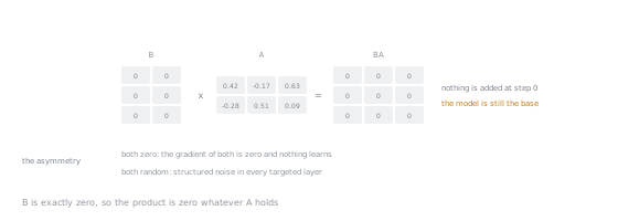
A's entries are visible and none of them matter: every one of them is multiplied by a zero on its way into the product.
The asymmetry is necessary. If both were zero, the gradient of both would be zero and nothing would ever learn: the product needs one factor non-zero to carry signal. If both were random, ΔW would start as structured noise injected into every targeted layer.
This is also why LoRA tolerates much higher learning rates than full fine-tuning. You are not nudging weights that already encode everything the model knows; you are growing a term from zero.
Alpha and the scaling factor
α (lora_alpha) is a fixed scalar. The update is scaled by α/r.
The point of dividing by r was to make the effective update magnitude roughly independent of rank, so that changing rank would not force you to re-tune the learning rate. What matters is the ratio α/r, not either number alone.
r | α | α/r | Effect |
|---|---|---|---|
| 8 | 16 | 2.0 | Common baseline |
| 16 | 32 | 2.0 | More capacity, same update scale |
| 16 | 16 | 1.0 | More capacity, weaker update |
| 64 | 16 | 0.25 | Much more capacity, heavily damped |
That last row is a trap worth naming: raising rank while leaving α fixed reduces the scale of the update. People raise rank hoping for more expressive power, forget α, and conclude that higher rank hurts. It did not; they quietly turned the adapter down by 8×.
The conventional starting point is α = 2r. Treat it as a convention with a rationale, not a discovery.
rsLoRA (arXiv:2312.03732) argues the α/r divisor over-damps at high rank and proposes α/√r instead, which keeps learning stable as rank grows. If you plan to work at rank 64 or above, this is the setting to know:
LoraConfig(r=64, lora_alpha=16, use_rslora=True, ...)
Choosing rank
Rank is capacity. It bounds how complex an update the adapter can express.
| Rank | Reasonable for |
|---|---|
| 4 to 8 | Style, tone, output format; small datasets |
| 16 to 32 | A genuine task with a few thousand examples |
| 64 to 128 | Harder tasks, larger datasets, reasoning-heavy behaviour |
| 256+ | Approaching full fine-tuning capacity on large SFT datasets |
Two diagnostics that beat guessing:
Underfitting. Training loss plateaus above where you need it and more epochs do not help. Not enough capacity: raise rank, or add target modules (usually the better move, per Lesson 10).
Overfitting. Training loss keeps falling while held-out loss rises. Too much capacity for the data, or too many epochs. Lower rank, add dropout, get more data, or stop earlier.
Note the asymmetry with the memory lesson: rank costs very little memory (Lesson 7), so the cost of extra rank is overfitting risk and a little compute, not fitting in memory. That inverts the instinct many people bring from the era when memory was the binding constraint.
Dropout
lora_dropout applies dropout to the adapter input. Typical values are 0.0 to 0.1. Reach for it when held-out loss is rising and you cannot get more data. On large datasets it is often unnecessary and simply slows convergence.
The config
config := {
    rank: 16,
    alpha: 32,               # α/r = 2
    dropout: 0.05,
    adapt_bias: false,
    target_modules: [...],   # Lesson 10
}

model := attach_adapter(model, config)
print(model.trainable_parameter_count())
That last line is not optional. It is the check that your target modules matched anything at all, and it should agree with the arithmetic you did in Lesson 8. Read the parameter names from the installed version's documentation rather than from memory, because this surface changes between releases.
Practice
- ▢ Why is
Binitialised to zero andArandomly, rather than both to zero or both randomly?
Check
Zero B makes ΔW = 0 at the start, so training begins from exactly the base model with no perturbation to recover from. Random A keeps the product's gradient non-zero, so learning can begin.
Both zero: gradients vanish, nothing learns. Both random: the model starts as base-plus-noise in every targeted layer.
- ▢ You raise rank from 8 to 64 and leave
αat 16. Loss barely moves. Diagnose.
Check
The scale α/r fell from 2.0 to 0.25. The adapter has eight times the capacity and one eighth the influence, so the net effect is a damped update, not a stronger one.
Raise α to 128 to preserve the ratio, or set use_rslora=True so the divisor becomes √r.
- ▢ Training loss flattens at a level too high to be useful, and a fourth epoch does not help. What is this, and what are your two options?
Check
Underfitting: the adapter lacks the capacity to express the required update.
Raise rank, or extend the target modules to cover more of the model. Adding target modules is usually the better first move, because the MLP holds most of the parameters and is often where the missing capacity is. More epochs cannot fix a capacity ceiling.
-
▢ Which pairing gives the strongest update scale?
- a)
r = 8withalpha = 8 - b)
r = 8withalpha = 32 - c)
r = 32withalpha = 32 - d)
r = 64withalpha = 64
- a)
Check
b) r = 8 with alpha = 32, giving α/r = 4.
The others are all α/r = 1. Capacity differs between them, but update scale does not, which is exactly the distinction the α/r design was meant to make.
- ▢ Why can LoRA use a learning rate ten to a hundred times higher than full fine-tuning?
Check
The trainable parameters start at zero contribution and are not themselves the store of pretrained knowledge. There is no accumulated structure to damage, and the term has to grow from nothing, so it needs a much larger step to move meaningfully within a reasonable number of steps.
- ▢ When would you not increase rank even though the adapter is underfitting?
Check
When the dataset is small. Extra capacity on few examples buys memorisation, not generalisation: training loss falls, held-out loss rises.
The right response there is more or better data, or a narrower task, not a bigger adapter.
Real-world reps
- [ ] Build three configs,
(8, 16),(16, 32)and(64, 16), and write down theα/rfor each and what you predict will happen. Keep the predictions. - [ ] Print
print_trainable_parameters()for each and reconcile against your Lesson 8 arithmetic. - [ ] Tomorrow: find a published fine-tuning config in the wild, work out its
α/r, and decide whether the author chose it or inherited it.
Going further
- Docs: LoRA, Hugging Face PEFT
- Paper: "A Rank Stabilization Scaling Factor for Fine-Tuning with LoRA", Kalajdzievski, arXiv:2312.03732
- Blog: "Practical Tips for Finetuning LLMs Using LoRA", Sebastian Raschka
- LoRA hyperparameters
Not landing? Reread the primary source at the top, since this lesson compresses it and compression is where understanding leaks. Check the glossary for any term that felt slippery.
If the lesson itself is unclear rather than the material, that is a defect: open an issue.