Lesson 26. Cost, Latency and Throughput
Mission link: "Measure what it cost in quality and latency" is on the success list. Fine-tuning is frequently a cost decision, and this is the arithmetic behind it.
Primary source: Blog: "LLM Inference Performance Engineering: Best Practices", Databricks
Prerequisites: Lesson 25
Warm-up
- ▢ What is the operational argument for unmerged serving?
Check
Rollback is a routing change rather than a deployment, and the untouched base stays available as a fallback and comparison point.
- ▢ Why must you evaluate the artifact you ship?
Check
Serving-time quantisation carries a permanent per-request quality cost. Numbers from a bf16 model do not describe a 4-bit deployment.
- ▢ What is fine-tuning bad at teaching?
Check
New facts, absent reasoning ability, current information, precise calculation.
Know this
The two-phase shape of inference
Generation has two phases with completely different performance characteristics, and confusing them makes every optimisation discussion incoherent.
Prefill processes the whole input prompt at once. All tokens are available, so the work is large parallel matrix multiplication, making it compute-bound. Cost scales with prompt length.
Decode generates one token at a time, each depending on the last. Each step reads the entire model's weights to produce a single token, so the arithmetic per byte moved is tiny, making it memory-bandwidth-bound. Cost scales with output length.
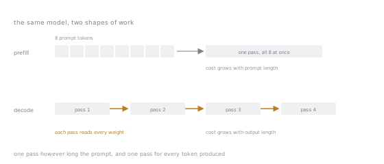
One box on the top row against four on the bottom is the whole asymmetry. Lengthening the prompt widens the single pass; lengthening the output adds boxes to the chain.
Consequences:
- Long prompts are cheap per token; long outputs are expensive per token. Not symmetric, and the asymmetry is large.
- Decode speed is set by memory bandwidth, so a smaller model is faster almost in proportion to its size.
- Batching helps decode enormously, because the weights are read once for the whole batch, and helps prefill much less.
The metrics that matter
| Metric | Meaning | Set by |
|---|---|---|
| Time to first token | Prefill latency | Prompt length, compute |
| Inter-token latency | Time per output token | Memory bandwidth, model size |
| Total latency | End to end | Both, plus queueing |
| Throughput | Tokens/second across all requests | Batching efficiency |
| Cost per request | Money | Throughput and hardware cost |
Latency and throughput trade against each other via batch size. Larger batches raise throughput and raise per-request latency. There is no single best setting: it depends on whether a human is waiting.
Where fine-tuning changes the economics
This is the part people miss. Fine-tuning's cost benefit usually has nothing to do with the weights being better.
Shorter prompts. A fine-tuned model needs no few-shot examples, no lengthy format instructions, no elaborate system prompt, because that behaviour is in the weights. If your prompt drops from 2,000 tokens to 200, you removed 1,800 tokens of prefill from every single request, forever. On a high-volume endpoint that is often the entire business case.
Shorter outputs. A model trained to answer in the required format stops padding with preamble and hedging. Since decode is the expensive phase, cutting output length is worth more per token than cutting input length.
A smaller model becoming sufficient. The strongest version of the argument: a fine-tuned small model that matches a general large model on your narrow task is dramatically cheaper per request and lower latency, because decode is bandwidth-bound and bandwidth scales with size. Trading a large general model for a small specialised one is where the order-of-magnitude savings live.
Fewer retries. If the general model produces invalid output 15% of the time and you retry, your true cost is 1.15× the visible cost. A fine-tune that reaches 99% validity removes almost all of that.
The honest accounting
Against those savings, count the costs:
| Cost | Nature |
|---|---|
| Training compute | One-off per version, usually small for adapters |
| Data creation | Often the dominant cost, and usually human time |
| Evaluation infrastructure | One-off, then ongoing maintenance |
| Serving complexity | Ongoing: adapter-capable stack, versioning, routing |
| Retraining | Ongoing: models, data and requirements all move |
| Expertise | Ongoing: someone must own this |
The recurring costs are what decide it, and they are the ones left out of the initial estimate. A fine-tune that saves a little money per request and requires a person to maintain it is a bad trade at low volume and a good one at high volume. The crossover is arithmetic, so do the arithmetic.
A worked comparison
Suppose a general large model with a 2,000-token prompt versus a fine-tuned small model with a 200-token prompt, both producing 150 output tokens.
General:  2000 prefill + 150 decode, on a large model
Tuned:     200 prefill + 150 decode, on a small model
The prompt saving is 1,800 prefill tokens. The model-size saving applies to both phases and especially to decode's bandwidth cost. Multiply by request volume, compare against the fixed and recurring costs above, and you have an actual answer rather than an intuition.
At a thousand requests a day this may not repay the data work. At a million it very likely does. The volume is the deciding variable, and it is the one least often stated.
Measure, do not model
Everything above is the right shape and the wrong precision. Actual numbers depend on hardware, serving stack, batch size, sequence lengths and traffic pattern in ways no formula captures. Measure:
- Time to first token and inter-token latency, at your real prompt lengths
- Throughput at several batch sizes, to find your latency/throughput point
- Cost per thousand requests, at your real traffic shape
- The same three for the alternative you are comparing against
And measure under realistic load. A benchmark on one request at a time tells you nothing about a batched production endpoint, because batching is the dominant factor in throughput.
Practice
- ▢ Which phase is compute-bound, which is bandwidth-bound, and what follows?
Check
Prefill is compute-bound, because the whole prompt is processed in parallel. Decode is memory-bandwidth-bound, because each step reads all the weights to produce one token.
It follows that long prompts are relatively cheap per token, long outputs are expensive, batching helps decode far more than prefill, and smaller models speed up decode nearly in proportion to size.
- ▢ Your fine-tune cuts prompt length from 1,800 tokens to 150 and leaves output length unchanged. Where does the saving come from?
Check
Prefill: 1,650 fewer tokens of compute-bound work on every request. The behaviour formerly specified by few-shot examples and format instructions now lives in the weights.
This is frequently the whole economic case for fine-tuning, and it has nothing to do with the model being smarter.
-
▢ Which fine-tuning benefit produces the largest cost reduction?
- a) The prompt becoming shorter by a thousand tokens
- b) A smaller model becoming sufficient for the task
- c) The output becoming shorter by fifty output tokens
- d) The retry rate falling from fifteen percent to one
Check
b) A smaller model becoming sufficient for the task.
It reduces both phases at once, and decode, the expensive phase, scales with model size because it is bandwidth-bound. The others are real and additive, but a model-size change is multiplicative across everything.
- ▢ Which costs are most often omitted from the initial estimate?
Check
The recurring ones: retraining as models and requirements move, serving complexity, evaluation maintenance, and the expertise of a person who owns it.
Training compute is cheap for adapters and gets quoted. Ongoing human cost is expensive and gets forgotten, and it is usually what decides the question.
- ▢ You measure single-request latency and conclude your endpoint is fast enough. What is wrong?
Check
Production serves concurrent requests in batches. Batch size dominates both throughput and per-request latency, and a single-request measurement observes neither.
Measure under realistic concurrency, at several batch sizes, and pick your point on the latency/throughput curve deliberately.
- ▢ Same task, same saving per request, 500 requests a day versus 5 million. Same decision?
Check
No. The fixed and recurring costs of data creation, evaluation, serving complexity and maintenance are essentially independent of volume, while the savings scale with it.
At 500 a day the recurring human cost almost certainly dominates. At 5 million it is negligible against the savings. Volume is the deciding variable and belongs in the first sentence of the proposal.
Real-world reps
- [ ] Measure time to first token and inter-token latency for your model at your real prompt lengths.
- [ ] Measure throughput at batch sizes 1, 4, 16 and 64. Plot the latency/throughput trade and pick your point.
- [ ] Compute cost per thousand requests for your fine-tuned path and for the alternative. Include the recurring costs.
- [ ] Tomorrow: find the request volume at which your fine-tune breaks even. Compare it to your actual volume.
Going further
- Blog: "LLM Inference Performance Engineering: Best Practices", Databricks
- Docs: Optimization and tuning, vLLM
- Lesson 27. When Not to Fine-Tune
Not landing? Reread the primary source at the top, since this lesson compresses it and compression is where understanding leaks. Check the glossary for any term that felt slippery.
If the lesson itself is unclear rather than the material, that is a defect: open an issue.