title: 4. ANN Indexes: HNSW and IVF
description: Why vector search trades exactness for speed, and how IVF and HNSW each expose that trade-off as a tunable knob
type: lesson

Lesson 4. ANN Indexes: HNSW and IVF

Mission link: Stage 3 opens the moving-target part of the mission, standing up search over a real corpus: an index is what makes vector search fast enough to run at all, at the cost of a recall/latency trade-off this lesson names before lesson 5 makes it concrete in pgvector.
Primary source: Paper: "Efficient and Robust Approximate Nearest Neighbor Search Using Hierarchical Navigable Small World Graphs", Malkov and Yashunin, 2018
Prerequisites: Lesson 3, Chunk

Warm-up

▢ A corpus has 2 million chunks. Roughly how much storage does embedding it at 1536 dimensions in float32 take, compared to 256 dimensions?

Check

About 12.3 GB at 1536 dimensions versus about 2.0 GB at 256 dimensions, since bytes per vector scales linearly with dimension count (dimensions × 4 bytes).

▢ What does Matryoshka Representation Learning let you do to an embedding vector that a standard embedding model doesn't safely allow?

Check

Truncate it to fewer dimensions after training, with a bounded, predictable quality cost, since an MRL-trained model's prefixes are themselves meaningful embeddings. A standard model's dimensions aren't ordered by importance, so truncating one is unpredictable.

Know this

Why exact search doesn't scale

Finding a query's true nearest neighbors exactly means comparing it against every vector in the corpus. That's linear in corpus size: doubling the corpus doubles the search time, and at millions of chunks, brute-force comparison becomes too slow to run at query time. An approximate nearest neighbor (ANN) index accepts a small, controllable amount of inexactness, returning vectors that are very likely close to the true nearest neighbors, not guaranteed to be exactly them, in exchange for search times that don't scale linearly with corpus size.

IVF: search only the nearby clusters

IVF (inverted file index) partitions the vector space into clusters ahead of time (commonly via k-means), assigning each vector to its nearest cluster centroid. At query time, instead of scanning every vector, IVF searches only the nprobe clusters nearest the query, where nprobe is a tunable count. A low nprobe (searching just the single nearest cluster) is fast but risks missing true neighbors that happen to sit in a neighboring cluster near the boundary. A high nprobe (searching many or all clusters) approaches exact search's recall at exact search's cost. IVF also carries a one-time build cost: the clustering step needs a representative sample of the corpus's vectors to place centroids well.

HNSW: a navigable graph, searched top-down

HNSW (hierarchical navigable small world) builds a multi-layer graph instead of clusters: each vector is a node, connected to other nearby vectors by edges, with sparser layers on top enabling long jumps across the vector space and a dense bottom layer enabling precise local search. A query starts at the sparse top layer, greedily hops toward whichever connected node is closest, and descends layer by layer, refining its position until it reaches the dense bottom layer. The tunable knob here is ef_search, how many candidates the search keeps track of at each step: a low ef_search finds an answer fast but may settle for a locally good node that isn't the true nearest; a high ef_search explores more candidates, trading speed for recall, the same shape of trade-off nprobe makes for IVF.

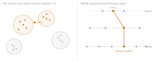
The general shape: a recall/latency curve, not a single right answer

Both indexes expose a knob (nprobe for IVF, ef_search for HNSW) that dials a specific point on a recall-versus-latency curve for a given corpus and index. HNSW generally lands on a better point of that curve than IVF, higher recall for the same latency, at the cost of more memory (the graph structure itself) and a slower index build. Neither index has one universally correct setting: the right point depends on the workload's latency budget and how much recall loss a later stage, such as reranking, can absorb without the final result suffering, which is exactly what stage 6's retrieval metrics exist to measure rather than assume.

Practice

▢ Why doesn't brute-force exact nearest-neighbor search scale to a corpus of millions of vectors, and what does an ANN index give up to fix that?

Check

Exact search compares the query against every vector, so its cost grows linearly with corpus size, becoming too slow at millions of vectors. An ANN index gives up the guarantee of finding the true nearest neighbors exactly, accepting a small, controllable chance of missing one, in exchange for search times that don't scale the same way.

▢ For an IVF index, describe what happens at each extreme of the nprobe parameter: nprobe = 1 versus nprobe set to search every cluster.

Check

nprobe = 1 searches only the single nearest cluster: fastest, but it can miss a true nearest neighbor sitting in a neighboring cluster near the boundary, especially if the query lands close to a cluster edge. nprobe set to search every cluster approaches exact search: highest recall, but at exact search's cost, since it no longer skips most of the corpus.

▢ How does HNSW's ef_search parameter play the same role for HNSW that nprobe plays for IVF?

Hint

Think about what each parameter controls: how much of the index gets examined before returning an answer.

Check

ef_search controls how many candidates the graph search keeps track of at each step while descending through HNSW's layers. A low value explores fewer candidates, finding an answer fast but risking settling for a node that isn't the true nearest. A high value explores more candidates, trading search speed for higher recall, the same recall-versus-latency shape nprobe gives IVF.

▢ What is the general trade-off between choosing HNSW and choosing IVF for a given corpus?

Check

HNSW typically achieves a better recall-for-a-given-latency point than IVF, but costs more memory (the graph's edges add real overhead beyond just storing the vectors) and takes longer to build the index in the first place. IVF is cheaper to build and store but generally needs to search a larger fraction of the corpus to match HNSW's recall at the same latency.

▢ Which claim is true of tuning an ANN index's search-time parameter (nprobe or ef_search)?
- a) There is one universally correct setting that works for any corpus and workload
- b) The right setting is a point on a recall/latency curve that has to be chosen against the workload's actual latency budget and tolerance for recall loss
- c) Setting the parameter as high as possible is always the right choice, since latency doesn't matter once an index exists
- d) The parameter only affects index build time, not query-time behavior

Check

b) Both parameters trade recall against latency at query time, and the right point depends on what the workload actually needs, which stage 6 measures rather than assumes. (a) is false: that's exactly what the recall/latency curve rules out. (c) is false: a higher setting costs more query-time latency, which matters whenever there's a latency budget to meet. (d) is false: both nprobe and ef_search are search-time parameters, not build-time ones.

Real-world reps

[ ] Find the index type (IVF or HNSW) your vector store uses or defaults to, and locate its search-time recall/latency parameter in its documentation.
[ ] If you can run queries against an index, try two different nprobe or ef_search values and observe the difference in query latency.
[ ] Tomorrow: read one paragraph of the HNSW paper's description of its layered structure and note, in your own words, why the top layer needs to be sparse for long-range jumps to work.

Going further

Not landing? Reread the primary source at the top, since this lesson compresses it and compression is where understanding leaks. Check the glossary for any term that felt slippery.

If the lesson itself is unclear rather than the material, that is a defect: open an issue.