Lesson 10. The Backward Pass and Autograd

Mission link: Lesson 9's scalar loss is useless to training on its own; the backward pass is what turns it into a gradient for every single weight in the model, which is the actual signal the optimizer (lesson 11) uses to improve them.
Primary source: Docs: "Autograd mechanics", PyTorch
Prerequisites: Lesson 9, Scaled dot-product attention

Warm-up

1. ▢ Why does cross-entropy use -log(p) rather than something like 1 - p as its penalty for a wrong prediction?

2. ▢ Why do residual connections help train a deep stack of transformer blocks?

Know this

Every forward operation records how it was computed

As the forward pass runs, every operation, a matrix multiply, a softmax, an addition for a residual connection, is recorded into a computation graph: a record of exactly which operation produced each intermediate tensor, and from which input tensors. This graph is what the backward pass walks, in reverse, to compute the gradient of the final scalar loss with respect to every tensor that contributed to it, all the way back to every trainable weight.

The chain rule, applied automatically

The mechanism underneath is nothing more than the calculus chain rule, automated: the gradient of the loss with respect to some tensor is the sum, over every path downstream of it in the graph, of the gradient of the loss with respect to that downstream tensor, multiplied by the local derivative of the downstream tensor with respect to this one. A concrete numeric case: let y = 3x + 1 and z = y^2. At x = 2, y = 7. dz/dy = 2y = 14. dy/dx = 3. By the chain rule, dz/dx = dz/dy × dy/dx = 14 × 3 = 42. Autograd does exactly this kind of multiplication and summation, just across every operation in a network with millions or billions of parameters instead of two small equations.

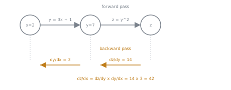
Automatic differentiation, not symbolic or numerical

PyTorch's autograd is neither symbolic differentiation (deriving a closed-form gradient formula by hand or via computer algebra) nor numerical differentiation (approximating a gradient with finite differences, which is imprecise and requires re-running the forward computation many times per parameter). Instead, every primitive operation (matrix multiply, addition, softmax, and so on) has a hand-derived local backward rule already implemented, and autograd chains those local rules together automatically, following the recorded computation graph, to produce exact gradients in a single backward traversal.

Where residual connections actually do their work

Lesson 5 argued residual connections keep gradients flowing through a deep stack; the chain rule is exactly where that argument becomes mechanical. For a residual output y = x + Sublayer(x), the gradient of the loss with respect to x is d(loss)/d(y) × 1 (the identity path's local derivative, which is exactly 1) plus a second term flowing through Sublayer's own local derivative. No matter how small or poorly behaved Sublayer's own local derivative becomes, that first term guarantees at least the direct, unscaled d(loss)/d(y) contribution passes through to x unchanged. This is the precise, mechanical reason residual connections prevent vanishing gradients, not just an informal intuition about "shortcuts."

One call populates every parameter's gradient

After the scalar loss is computed, a single call, loss.backward(), traverses the entire computation graph and accumulates, into every trainable parameter's .grad attribute, the gradient of the loss with respect to that parameter. Gradients accumulate by default rather than overwrite, adding into whatever was already in .grad, which is why a training loop has to explicitly zero every parameter's gradient before each new backward pass; otherwise, each step's gradient would be contaminated by the previous step's leftover values.

Practice

1. ▢ Let y = 3x + 1 and z = y^2. At x = 2, compute y, dz/dy, dy/dx, and dz/dx using the chain rule.

2. ▢ For a residual output y = x + Sublayer(x), what term does the identity path contribute to d(loss)/d(x), and why does this guarantee some gradient reaches x regardless of how small Sublayer's own local derivative is?

3. ▢ Why is automatic differentiation (autograd) preferred over numerical differentiation (finite differences) for training a large network?

4. ▢ What does calling loss.backward() actually populate, and why must gradients typically be zeroed before the next call?

5. ▢ Which claim is true of autograd's approach to computing gradients?

   • a) It requires the user to derive and supply a closed-form gradient formula for each operation
   • b) It approximates gradients using finite differences, perturbing each parameter slightly
   • c) It records the forward pass's operations into a computation graph, then applies the chain rule automatically using each operation's already-implemented local backward rule
   • d) It computes gradients only for the final output layer, not for earlier layers in a deep stack

Real-world reps

• [ ] Build a small computation graph by hand (two or three chained operations, like the worked example) and verify PyTorch's autograd produces the same gradient your manual chain-rule calculation does.
• [ ] Run a forward pass, call loss.backward() twice in a row without zeroing gradients in between, and confirm the second call's .grad values reflect accumulation rather than a fresh gradient.
• [ ] Tomorrow: read the "How autograd encodes the history" section of the primary source docs and note how the recorded graph differs between a fresh forward pass and one run with gradient tracking disabled.

Going further

• Docs: "Autograd mechanics", PyTorch
• Repo: nanoGPT, Karpathy
• Resources

Not landing? Reread the primary source at the top, since this lesson compresses it and compression is where understanding leaks. Check the glossary for any term that felt slippery.

If the lesson itself is unclear rather than the material, that is a defect: open an issue.