Lesson 9. Aggregation and GROUP BY

Mission link: A total from a joined query is arithmetic over whatever rows the join produced, and a join producing three rows per real fact makes the total three times too big, with no error and nothing that looks wrong. This lesson gives the rules an aggregate follows, so that number is right before it reaches a report.
Primary source: PostgreSQL, 2.7 Aggregate Functions
Prerequisites: Lesson 2, Lesson 8

Warm-up

1. ▢ Lesson 8 grouped a left join per customer and found that customer 6, who has no orders, gave count(*) a value of 1 and count(o.id) a value of 0 for the same row. Why do the two disagree?

Know this

An aggregate collapses a set of rows to one value, and ignores NULL except in count(*)

orders has 12 rows, and amount is NOT NULL on all of them, but shipped_at is missing on four:

SELECT count(*) AS n, count(shipped_at) AS shipped, sum(amount) AS total, avg(amount) AS mean
FROM orders;

n  | shipped | total   | mean
---+---------+---------+---------------------
12 | 8       | 2406.49 | 200.5408333333333333

count(*) is the row count, 12. count(shipped_at) is 8, because it counts values rather than rows, and orders 103, 105, 108 and 110 have never shipped. sum and avg here run over all twelve amounts, since amount has nothing missing to skip. The skip only becomes visible once a column actually has gaps:

SELECT avg(x) AS mean, count(*) AS n, count(x) AS present
FROM (VALUES (10), (20), (NULL)) AS v(x);

mean                | n | present
--------------------+---+--------
15.0000000000000000 | 3 | 2

Three rows, but the mean is 15, not 10. avg divides by the count of values it saw, 2, not by the row count, 3: an absent value is treated as not part of the calculation, not as a zero. Every aggregate here except count(*) behaves this way.

Aggregating over no rows at all is not the same as aggregating over zero

SELECT count(*) AS n, sum(amount) AS total, avg(amount) AS mean
FROM orders WHERE amount > 100000;

n | total | mean
--+-------+-----
0 |       |

count(*) is 0, correctly. sum and avg come back NULL, also correct in a narrow sense, since there is nothing to sum or average. What it costs a caller is real: a blank cell looks like the query failed rather than like nothing qualified. coalesce fixes it where the result meets whatever prints it:

SELECT coalesce(sum(amount), 0) AS total FROM orders WHERE amount > 100000;

total
-----
0

count(*) never needs this; every other aggregate over an empty set gives NULL, and a report that prints an empty total as blank rather than as zero is a bug a user sees.

GROUP BY puts every NULL into one group, the opposite of what WHERE and a join do

SELECT c.country, count(*) AS n, sum(o.amount) AS total
FROM customers c
JOIN orders o ON o.customer_id = c.id
GROUP BY c.country
ORDER BY c.country;

country | n | total
--------+---+--------
GB      | 4 | 260.75
JP      | 2 | 365.75
NL      | 1 | 60.00
US      | 3 | 1019.99
        | 2 | 700.00

Five groups, not four. Customers 2 and 8 both have country IS NULL, and rather than being dropped, they land in one group together, 2 orders and 700.00. Lesson 3 established that NULL = NULL is unknown, which is why WHERE country = 'GB' and a join condition both refuse to match a NULL. GROUP BY is not asking that question: it partitions rows into buckets, and every unknown value gets the same bucket, purely so grouping has somewhere to put rows it cannot compare. That is deliberate, not an inconsistency between two features that disagree.

The column has to survive the collapse, and a key makes it survive anyway

SELECT c.country, c.email, count(*)
FROM customers c
JOIN orders o ON o.customer_id = c.id
GROUP BY c.country;

ERROR:  column "c.email" must appear in the GROUP BY clause or be used in an aggregate function
SQLSTATE: 42803

Lesson 2 put GROUP BY before SELECT in the evaluation order, and that is the whole explanation rather than a rule to memorise separately. By the time SELECT runs, the GB rows have already collapsed into one group of four, and those four rows carry different emails; there is no single row left to read c.email from, so PostgreSQL refuses rather than picking one arbitrarily.

A primary key survives this without complaint:

SELECT c.id, c.email, count(*)
FROM customers c
JOIN orders o ON o.customer_id = c.id
GROUP BY c.id
ORDER BY c.id
LIMIT 3;

id | email             | count
---+-------------------+------
1  | ada@example.com   | 3
2  | grace@example.com | 1
3  | alan@example.com  | 1

Grouping by c.id and selecting c.email is accepted, because id determines exactly one row, and therefore exactly one email, leaving nothing ambiguous even though email is neither grouped nor aggregated. Grouping positionally, and grouping by a SELECT alias, both work too, and PostgreSQL accepts them; that is not a claim about a standard:

SELECT c.country AS ctry, count(*) FROM customers c JOIN orders o ON o.customer_id = c.id GROUP BY 1;
SELECT c.country AS ctry, count(*) FROM customers c JOIN orders o ON o.customer_id = c.id GROUP BY ctry;

ctry | count
-----+------
GB   | 4
JP   | 2
NL   | 1
US   | 3
     | 2

Both statements return that same five-row result. Filtering groups by a count is HAVING, next lesson's subject.

The fan-out bug

This is the section this lesson exists for. Joining customers to orders and then to countries, filtering only on the country's own region rather than on any relationship between a customer and that country:

SELECT count(*) AS n, sum(o.amount) AS total
FROM customers c
JOIN orders o ON o.customer_id = c.id
JOIN countries n ON n.region = 'Europe';

n  | total
---+--------
36 | 7219.47

Thirty six rows, and 7219.47 against a true total of 2406.49, exactly three times too big. Three country rows, GB, DE and FR, satisfy region = 'Europe', and the join never relates a specific customer or order to a specific country, so every order survives once per matching country. The rule is arithmetic: a join that multiplies rows multiplies every additive aggregate built on it, sum and count(*) alike, by exactly the row multiplier, since both are addition run once per surviving row. avg came out unaffected, 200.5408333333333333, because its numerator and denominator scaled by three and cancelled; that is a coincidence of an even fan-out, not something to rely on.

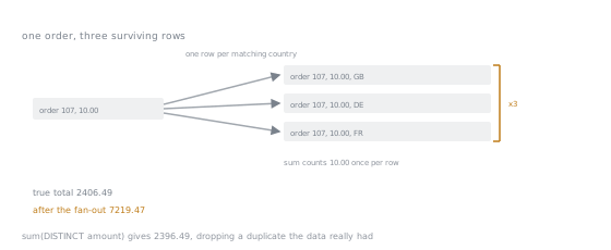
Every additive aggregate runs once per surviving row, so the multiplier on the right of the fan is the multiplier on the total: 2406.49 times three is 7219.47, with nothing in between to notice.

The instinctive repair fails, and it is worth seeing why:

SELECT sum(DISTINCT o.amount) AS wrong
FROM customers c
JOIN orders o ON o.customer_id = c.id
JOIN countries n ON n.region = 'Europe';

wrong
-------
2396.49

Wrong by a smaller, more dangerous margin. Orders 107 and 108 are both genuinely 10.00, and DISTINCT on the amount collapses that real duplicate into one value. No DISTINCT on the output repairs a fan-out: DISTINCT removes rows that are identical, and it cannot tell a duplicate the join manufactured from a duplicate that was always true of the data.

Two fixes work. Aggregate before joining, so the fact table is already collapsed before anything can multiply it:

SELECT sum(pre.total) AS grand_total
FROM (
    SELECT customer_id, sum(amount) AS total
    FROM orders
    GROUP BY customer_id
) pre;

grand_total
-----------
2406.49

Or aggregate over values that identify the original row, not over the value being summed:

SELECT count(*) AS n, sum(order_amount) AS total
FROM (
    SELECT DISTINCT o.id AS order_id, o.amount AS order_amount
    FROM customers c
    JOIN orders o ON o.customer_id = c.id
    JOIN countries n ON n.region = 'Europe'
) d;

n  | total
---+-------
12 | 2406.49

Reach for aggregating before joining first: it fixes a sum, a count and an avg alike. Distinct-on-the-key only rescues a query genuinely about distinct rows, and only when it keys on an actual identifier, not on the value itself, as the wrong 2396.49 above shows.

Aggregating after an outer join, the fan-out's mirror image

The fan-out is too many rows standing in for one fact. An outer join can produce the opposite: a row standing for the absence of one.

SELECT n.region, count(*) AS star, count(c.id) AS cid
FROM countries n
LEFT JOIN customers c ON c.country = n.code
GROUP BY n.region
ORDER BY n.region;

region   | star | cid
---------+------+----
Africa   | 1    | 0
Americas | 3    | 2
Asia     | 2    | 1
Europe   | 4    | 2

Africa has count(*) of 1, because Kenya's row survives the left join with no customer to pair it with, and count(c.id) of 0, because that row's c.id is NULL. One counts rows, the other counts customers, and only the second answers "how many customers are based in Africa". They agree wherever a country has a matching customer, and disagree exactly where the left join kept a country that would otherwise have vanished, the warm-up's gap again, now at the level of a whole group.

Practice

1. ▢ Before running it, predict count(*), sum(amount) and avg(amount) for the orders where shipped_at IS NULL.

2. ▢ Predict the exact error and SQLSTATE of adding n.name to SELECT c.country, count(*) FROM customers c JOIN orders o ON o.customer_id = c.id JOIN countries n ON n.code = c.country GROUP BY c.country, without changing the GROUP BY.

3. ▢ Group the same join by c.id instead, keeping c.email in SELECT. Predict whether it errors, and say in one sentence why grouping by country and by id differ here.

4. ▢ Before running it, predict the row count and sum(o.amount) of the three-way join in this lesson that filters countries only on region = 'Europe', using the number of European rows in countries and the number of orders.

5. ▢ Fix the previous query by aggregating orders in a derived table before any join touches it. Predict the corrected total.

   SELECT sum(pre.total) AS grand_total
   FROM (SELECT customer_id, sum(amount) AS total FROM orders GROUP BY customer_id) pre;
   

6. ▢ Using this lesson's countries LEFT JOIN customers grouping by region, predict count(*) and count(c.id) for Americas, and say which one answers "how many customers are based in the Americas".

Real-world reps

• [ ] Find a report query at work that sums or counts across a join, and check by hand whether that join can produce more than one row per fact it is meant to count.
• [ ] Find a total that renders as a blank cell when nothing matched, and decide whether a zero would have told its reader the truth better.
• [ ] Tomorrow: pick a GROUP BY query you or a colleague wrote recently, and for every unaggregated column in SELECT, check whether it is there because of a primary key or because it happened to work by luck.

Going further

• 2.7 Aggregate Functions: the tutorial this lesson compresses
• 9.21 Aggregate Functions: the complete reference list of built-in aggregates, and which ones treat NULL differently from count(*)
• 7.2.4 GROUP BY and HAVING: the grammar for GROUP BY, ahead of HAVING in the next lesson
• Querying: the stage 2 reference sheet
• Resources

Not landing? Reread the primary source at the top, since this lesson compresses it and compression is where understanding leaks. Check the glossary for any term that felt slippery.

If the lesson itself is unclear rather than the material, that is a defect: open an issue.