Lesson 36. What an Index Actually Does
Mission link: A query that scans a growing table gets slower in a straight line, and the fix is rarely a faster machine but a structure turning that scan into a lookup, which means reading what a plan says it actually did.
Primary source: PostgreSQL, Chapter 11 Indexes
Prerequisites: Lesson 29, Lesson 35
Warm-up
- ▢ Lesson 35 read a plan for
select count(*) from orders where customer_id = 4242with no index anywhere nearcustomer_id, and the node doing the work reportedRows Removed by Filter: 349970besiderows=2.33 loops=3. What does that number actually count, and what would have to be true of the table for it to be small instead of large?
Check
Every row a worker read and threw away because customer_id did not equal 4242, out of about 350,000 rows per worker. It is large because nothing points the scan at customer 4242's seven rows, so finding them means looking at all of them; it would shrink only if the table itself did, which an index changes without touching the table's size at all.
Know this
What a B-tree is, in the two sentences that matter
A B-tree is a sorted, balanced structure whose interior pages narrow a search, and whose leaf pages hold the indexed values in order, each with a pointer to its row, so finding a value costs a walk of a few pages rather than a read of the whole table. The consequence worth checking in a plan is not the lookup itself but that the same ordering makes a range and a sorted read possible too: an index built for customer_id = 4242 also answers customer_id between 4242 and 4400 and order by customer_id, because the leaves were already in that order.
The four ways a plan says it read a table
Every scan of orders here resolves to one of four nodes. Seq Scan, or its parallel form under a Gather, reads every page in physical order, the fallback when nothing narrows the search, as the warm-up showed; build create index i36_customer_id on orders (customer_id) and it stops appearing for that predicate. Index Scan walks the B-tree to matching leaf entries, then visits the heap once per match, forced by a column the index does not store. Index Only Scan walks the same tree but answers from the leaf entries alone, reporting Heap Fetches: 0 when the heap is never touched, the next section's subject. Bitmap Heap Scan, the fourth, needed building on purpose: a column the index lacks, over a predicate matching enough scattered rows that visiting them one at a time costs more than visiting their pages in order.
Finalize Aggregate (actual rows=1.00 loops=1)
  Buffers: shared hit=6808 read=800
  ->  Gather (actual rows=3.00 loops=1)
        ->  Partial Aggregate (actual rows=1.00 loops=3)
              ->  Parallel Seq Scan on orders (actual rows=2.33 loops=3)
                    Filter: (customer_id = 4242)
                    Rows Removed by Filter: 349970
                    Buffers: shared hit=6808 read=800
The seq scan again, 7608 buffers total however this run split them between cache and disk. Against amount, correlation close to zero, select id from orders where amount between 200 and 220 matches 42039 of 1,049,916 rows, about four percent, scattered rather than clustered:
Bitmap Heap Scan on orders (actual rows=42039.00 loops=1)
  Recheck Cond: ((amount >= '200'::numeric) AND (amount <= '220'::numeric))
  Heap Blocks: exact=392
  Buffers: shared hit=510
  ->  Bitmap Index Scan on i36_amount (actual rows=42039.00 loops=1)
        Index Cond: ((amount >= '200'::numeric) AND (amount <= '220'::numeric))
        Buffers: shared hit=118
The child collects every matching entry first, then the parent visits the heap page by page, Heap Blocks: exact=392, instead of jumping row to row; 510 buffers for 42039 rows beats 42039 separate random heap visits, the whole reason the node exists.
Why an index-only scan is possible at all
The lesson's best idea: the index already holds the value asked about, so if the query needs nothing else, the table is never read. The proof runs one predicate, customer_id = 4242, once asking only for a count and once for a column the index does not contain:
Aggregate (actual rows=1.00 loops=1)
  Buffers: shared hit=7
  ->  Index Only Scan using i36_customer_id on orders (actual rows=7.00 loops=1)
        Index Cond: (customer_id = 4242)
        Heap Fetches: 0
        Index Searches: 1
Index Scan using i36_customer_id on orders (actual rows=7.00 loops=1)
  Index Cond: (customer_id = 4242)
  Index Searches: 1
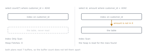
Both find the same seven rows at 7 buffers, but the second is select id, amount from orders where customer_id = 4242, and amount is not in i36_customer_id, so it drops the word Only.
The whole difference is whether that arrow exists. It is not a difference in how much work the index did, which is why the buffer count is the same on both sides and cannot be used to tell them apart. Heap Fetches: 0 answers the real question, not the buffer count, since a heap fetch and an index-only page can both cost one buffer. Lesson 29's caveat still applies: visibility lives in the table, not the index, so an index-only scan still checks a visibility map before trusting a leaf entry alone. A five-thousand-row scratch table shows the mechanism directly, one row updated with no VACUUM in between:
Index Only Scan using i36_demo_val on demo (actual rows=1.00 loops=1)
  Heap Fetches: 0
  Buffers: shared hit=3

-- after: UPDATE demo SET val = val WHERE id = 2500, no VACUUM run since

Index Only Scan using i36_demo_val on demo (actual rows=1.00 loops=1)
  Heap Fetches: 1
  Buffers: shared hit=4
Heap Fetches above zero on a table with a recent write is that visibility check showing through, not a mistake: the page holding row 2500 no longer counts as all-visible, so the scan opens the heap once to check, the same mechanism lesson 29 described for a snapshot, here showing through an index.
When an index stops helping
Widen the predicate from 159 customers to customer_id < 50000, about half the table, and the honest version of "an index stops helping" is not a switch back to a sequential scan:
Finalize Aggregate (actual rows=1.00 loops=1)
  Buffers: shared hit=8 read=579
  ->  Gather (actual rows=3.00 loops=1)
        ->  Partial Aggregate (actual rows=1.00 loops=3)
              ->  Parallel Index Only Scan using i36_customer_id on orders (actual rows=174971.67 loops=3)
                    Index Cond: (customer_id < 50000)
                    Heap Fetches: 0
The planner keeps the index and parallelises, 587 buffers against the narrow range's 9. That choice is cost, not instinct: random_page_cost, default 4, charges four times seq_page_cost's 1 for a page reached out of order, and against half a table the index still wins that arithmetic once split three ways. Change either setting and the crossover point moves with it.
The other index types, honestly
B-tree is the one to reach for; the other four earn their place only for the data shapes they name. Hash stores a 32-bit hash of the value and answers only "does this exact value exist," nothing about order: with i36_customer_id dropped and create index i36_customer_id_hash on orders using hash (customer_id) in its place, the equality query still finds its seven rows, but through a Bitmap Heap Scan rather than a plain Index Scan, since a hash carries no page ordering and no stored value to answer from alone:
Bitmap Heap Scan on orders (actual rows=7.00 loops=1)
  Recheck Cond: (customer_id = 4242)
  Heap Blocks: exact=1
  Buffers: shared hit=6
  ->  Bitmap Index Scan on i36_customer_id_hash (actual rows=7.00 loops=1)
        Buffers: shared hit=5
The same range the B-tree served earlier, customer_id between 4242 and 4400, falls back to the Parallel Seq Scan from the first section with only the hash index present, since a hash has no ordering for a range to walk. GIN answers "does this row contain this element," an inverted index for a column with many components, array entries or lexemes. GiST answers "what overlaps or lies nearest to this shape," geometric containment and nearest-neighbour search. SP-GiST answers the same kind of question over data that partitions naturally rather than sorts. BRIN answers "which block range could hold this value," a summary that pays off only when a column already sits near its neighbours on disk. Each of the four is a bet on a shape a B-tree lacks.
The cost of an index
Every index is another structure a write has to maintain, and another block of storage worth reading rather than guessing at: pg_relation_size('orders') returns 62324736 bytes, 59 MB, for the table itself, and pg_relation_size('i36_amount'), the B-tree built earlier on amount alone, came to 23 MB. That is real space holding nothing a query could not, in principle, get from the table. What that costs write throughput is lesson 41's measurement; here it is only what a reader can read directly off disk.
Practice
- ▢ The warm-up's
Rows Removed by Filter: 349970came from a table with no index nearcustomer_id. Predict what number in the plan takes over as "how much work this did" oncei36_customer_idexists, and predict its value for customer4242.
Check
rows=7.00 on the Index Only Scan node, since customer 4242 has exactly seven orders and the scan visits only matching entries; there is no Rows Removed by Filter any more, because the index never hands the executor a non-matching row to discard.
- ▢
i36_customer_idindexescustomer_idalone. Predict whetherselect id, amount from orders where customer_id = 4242runs asIndex Only Scanor plainIndex Scan, and name the one word in the plan that gives it away.
Hint
Ask which of id or amount the index on (customer_id) actually stores.
Check
Plain Index Scan, because amount is not in the index, so the row has to come from the heap regardless of how cheap the lookup was; the tell is the missing word Only, not a number.
- ▢ With only
i36_customer_id_hashin place, no B-tree, predict whatselect count(*) from orders where customer_id between 4242 and 4400does, given that a hash index stores nothing but a 32-bit hash per value.
Check
It falls back to Parallel Seq Scan, the node the first section showed with no index at all. A hash carries no ordering between values, so between has nothing to walk; only = can reach a hash index.
- ▢ Two indexes were built on the same 1,049,916 rows of
orders, a B-tree onamountand a hash oncustomer_id. Predict which one takes more space on disk.
Hint
Compare what each structure has to store per entry, not which column's values look larger.
Check
The hash index, 32 MB against the B-tree's 23 MB. customer_id is a smaller value than amount, but a hash index's bucket layout carries more overhead per entry than a B-tree's densely packed leaf pages, so the difference is about structure, not data type.
- ▢ A five-thousand-row table gave
Heap Fetches: 0on anIndex Only Scan, then one row was updated with noVACUUMrun afterwards. Predict what the same query'sHeap Fetchesreads on the very next run.
Check
1, not 0. The update left that row's page no longer marked all-visible, so the scan opens the heap once to confirm visibility before trusting the leaf entry; that fetch is the visibility map doing its job, not a regression.
- ▢
select id from orders where amount between 200 and 220matches about four percent of the table, scattered rather than clustered byamount. Predict whether the plan is a plainIndex Scanor aBitmap Heap Scan, and which single number in the plan explains the choice.
Hint
Ask what a plain Index Scan would do between one matching row and the next, given they are scattered rather than neighbours.
Check
Bitmap Heap Scan, and Heap Blocks: exact=392 explains it: visiting 392 heap pages once each, in order, beats 42039 separate random single-row lookups, since scattered matches would otherwise mean revisiting pages already left behind.
Real-world reps
- [ ] Pick a query against a table of more than a few thousand rows and check which of the four scan kinds its
EXPLAIN (ANALYZE)names for the node reading it. - [ ] Find a query that already runs an
Index Only Scanand check itsHeap Fetches: nonzero on a table with recent writes is the visibility map at work, not a broken index. - [ ] Tomorrow: pick one column you filter on often with no nearby index, build one on a copy of the data, rerun the query, and compare only the buffer count before and after.
Going further
- 11.2. Index Types: every index type this lesson named, B-tree included
- 11.9. Index-Only Scans and Covering Indexes: the visibility map behind
Heap Fetches - 19.7.2. Planner Cost Constants:
random_page_cost,seq_page_costand the rest - Performance: the stage 6 reference sheet
- Resources
Not landing? Reread the primary source at the top, since this lesson compresses it and compression is where understanding leaks. Check the glossary for any term that felt slippery.
If the lesson itself is unclear rather than the material, that is a defect: open an issue.