Lesson 37. Selectivity and Statistics

Mission link: A query that goes from fast to slow with no code change usually still has a sensible plan for the wrong row count, and finding that means reading the statistics the planner read, not staring at the query again.
Primary source: PostgreSQL, 14.2. Statistics Used by the Planner
Prerequisites: Lesson 35, Lesson 36

Warm-up

1. ▢ Lesson 35 read a plan's rows= figure twice, once from a bare EXPLAIN and once, under ANALYZE, next to what actually happened, and treated a wide gap between the two as a sign that something upstream needed attention. Before a single row of the query is read, where does that first, printed-without-ANALYZE number come from?

Know this

Selectivity, and the cardinality it produces

Selectivity is the fraction of a table's rows a condition keeps; cardinality is the row count that follows from multiplying that fraction by the table's size. Neither word is in the glossary yet, so both are pinned here. Of the large fixture's 1,049,916 orders, customer_id = 4242 keeps a handful, and customer_id < 33334 keeps 349932, almost exactly a third. With an index on customer_id, EXPLAIN (ANALYZE) prints the planner's guess next to what happened for each:

Aggregate (actual rows=1.00 loops=1)
  -> Index Only Scan using i37_customer_id on orders (cost=0.43..12.61 rows=13 width=0) (actual rows=7.00 loops=1)
        Index Cond: (customer_id = 4242)

Finalize Aggregate (actual rows=1.00 loops=1)
  -> Gather (actual rows=3.00 loops=1)
        Workers Planned: 2
        -> Partial Aggregate (actual rows=1.00 loops=3)
              -> Parallel Index Only Scan using i37_customer_id on orders (cost=0.43..10358.80 rows=146198 width=0) (actual rows=116644.00 loops=3)
                    Index Cond: (customer_id < 33334)

rows=13 is almost double the actual rows=7.00, a harmless miss. rows=146198 is a per-loop figure; times three loops against 116644.00 times three, both sides land near 439000 estimated against 349932 actual. The plan's shape changed too: the tiny predicate stayed a single Index Only Scan, and the third-of-the-table predicate became a Gather over a Parallel Index Only Scan, because the planner's arithmetic, done before either query ran, told it roughly how much work each was.

Where the numbers come from

pg_stats on orders held these figures after one ANALYZE:

attname     | n_distinct  | correlation | most_common_vals | most_common_freqs
customer_id | 80112.0     | 0.96066135  | {54843}          | {0.0002}
shipped_at  | -0.3462353  | 0.06040191  |                  |
id          | -1.0        | 0.96066135  |                  |
amount      | 40224.0     | -0.02006983 | {475.20}         | {0.00023333334}

n_distinct's sign changes its meaning: positive, as customer_id's 80112, is an absolute headcount, here an underestimate of the true 100000 because ANALYZE samples rather than reads the table; negative, as id's -1.0, is minus the ratio of distinct values to rows, so -1 means one distinct value per row, right for a primary key, and shipped_at's -0.3462353 means roughly a third as many distinct timestamps as rows. most_common_vals is empty for id and shipped_at, and nearly so for customer_id and amount: every customer holds one to twenty orders and no value stands out, so nothing repeats often enough to be worth naming. The one entry that did surface, customer_id = 54843 claimed at frequency 0.0002, is a sampling artefact: its true frequency is about 0.000019, roughly ten times smaller, because the sample happened to see a few extra rows of that value. The histogram, 101 bounds from 1.01 to 500.97 for amount, divides its range into 100 roughly equal-frequency buckets, priced against by a range condition once most_common_vals does not cover it. correlation is 0.96, close to 1.0, for id and customer_id, since the generator inserted every customer's orders in order, and near zero, -0.02, for amount; it prices an index scan's cost, since rows an index visits in order sit together on disk near 1.0 and scattered near zero.

ANALYZE, and the sample it takes

Those numbers are a snapshot and go stale the moment the data moves without a fresh ANALYZE, shown here on a table of one's own rather than the shared fixture: a million rows, id and group_id set to id % 100000, giving each of 100,000 groups about ten rows, so group_id = 4242 analyses to a true count of 10 and a matching estimate. Inserting 5,000 more rows for group_id = 4242 moves the true count to 5010, but the stale estimate still reads the pre-insert figure:

-> Parallel Seq Scan on stale (cost=0.00..10667.34 rows=4 width=0) (actual rows=1670.00 loops=3)
      Filter: (group_id = 4242)

rows=4 per loop, unchanged, against an actual rows=1670.00 per loop, three loops of a true 5010 the stale statistics know nothing about. ANALYZE on that same table moves the estimate:

-> Parallel Seq Scan on stale (cost=0.00..10667.38 rows=2233 width=0) (actual rows=1670.00 loops=3)
      Filter: (group_id = 4242)

rows=2233 against the same actual rows=1670.00 is off by less than half rather than by two orders of magnitude. Autovacuum does the same job on its own schedule, queuing an automatic analyse once more than autovacuum_analyze_threshold (50 here) plus autovacuum_analyze_scale_factor (0.1) times the row count has changed since the last one. default_statistics_target, 100 by default and confirmed by the 101-entry histogram above, sets the sample size and how many most_common_vals and histogram entries ANALYZE keeps per column, and it can be raised for one column alone, back on the shared fixture: ALTER TABLE orders ALTER COLUMN customer_id SET STATISTICS 1000 then ANALYZE orders moved customer_id's n_distinct from 80112 to 91251, closer to the true 100000, and its customer_id = 4242 estimate from rows=13 to rows=11, against a true 7. A wider sample on the one column that needs it is the most useful move in this lesson.

The estimate the planner cannot get right alone

Every number so far describes one column at a time, and the planner assumes two conditions on two columns are independent, an assumption that fails when the columns move together. A scratch table of 100,000 rows, group_a and group_b both derived from the same value so one always determines the other, shows the failure cleanly:

Aggregate (actual rows=1.00 loops=1)
  -> Seq Scan on pairs (cost=0.00..2137.00 rows=1 width=0) (actual rows=100.00 loops=1)
        Filter: ((group_a = 'A0500'::text) AND (group_b = 'B0500'::text))

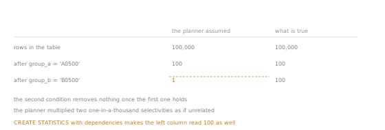
The two columns agree until the second condition, and the whole error is one step. Nothing is wrong with either selectivity on its own, which is why no single-column statistic can fix this and why the repair is an object that describes the pair.

The estimate, rows=1, is a hundred times smaller than the actual rows=100.00: the planner multiplied each column's one-in-a-thousand selectivity as if unrelated, when the second condition adds nothing once the first is true. CREATE STATISTICS i37_group_dep (dependencies, ndistinct) ON group_a, group_b FROM pairs, followed by another ANALYZE, tells the planner about the dependency directly:

Aggregate (actual rows=1.00 loops=1)
  -> Seq Scan on pairs (cost=0.00..2137.00 rows=100 width=0) (actual rows=100.00 loops=1)
        Filter: ((group_a = 'A0500'::text) AND (group_b = 'B0500'::text))

The same query now estimates rows=100, matching the actual count exactly. That fix only reaches equality conditions; the documentation is explicit that a dependencies object does nothing for a range condition or a LIKE, so the same misestimate returns the moment = becomes BETWEEN.

What a wrong estimate does downstream

A wrong row count rarely stays where it started. The node that expected about 12 rows and produced 5010 feeds that number to whatever runs next, and a join or an aggregate above it sizes its strategy and working memory against the number handed to it, not reality; lesson 39 covers that choice of join strategy, and this lesson stops short of teaching it. The symptom, a slow join or a sort spilling to disk, is often two plan levels above the estimate that caused it, so the first move on a surprising plan is finding the smallest node whose estimated and actual rows= disagree by an order of magnitude, not the node where the time was spent.

The limits of a sample

None of this makes an estimate exact. Raising amount's target from 100 to 1000 moved the estimate for amount BETWEEN 100 AND 102 from 5190 to 5244, against a true count of 4238, further away rather than closer, because a bigger sample is still a sample. ANALYZE runs before a single row of any later query is read, so every plan rests on a forecast, and the reader's job is noticing when that forecast is wrong by an order of magnitude, not chasing one a sample cannot deliver exactly.

Practice

1. ▢ Using the pg_stats row for id, where n_distinct reads -1.0, predict what n_distinct would read for a boolean column storing shipped_at IS NULL, and say why its sign differs from id's.

2. ▢ Predict which keeps the smaller fraction of orders, customer_id = 4242 or customer_id < 33334, and roughly how many rows each keeps.

3. ▢ The pairs demonstration fixed its misestimate with CREATE STATISTICS ... (dependencies, ndistinct) on an equality condition. Predict what the same statistics object buys a query written as group_a BETWEEN 'A0490' AND 'A0510' AND group_b BETWEEN 'B0490' AND 'B0510' instead.

4. ▢ After the bulk insert into the scratch table for group_id = 4242, the estimate stayed at rows=4 per loop while the true count had already become 5010. Predict whether running the same query again, with no ANALYZE in between, changes that estimate.

5. ▢ This server's autovacuum_analyze_threshold is 50 and its autovacuum_analyze_scale_factor is 0.1. Predict, in round numbers, how many changed rows on the 1,049,916-row orders table it takes before autovacuum queues an automatic ANALYZE.

6. ▢ Raising amount's statistics target from 100 to 1000 moved the amount BETWEEN 100 AND 102 estimate from 5190 to 5244, against a true count of 4238, further away rather than closer. Predict whether raising it again, to the maximum of 10000, reliably fixes that.

Real-world reps

• [ ] Pick a query you run often and check whether its WHERE clause has two conditions on columns that tend to move together; if so, that is this lesson's correlated-columns section waiting to happen to you.
• [ ] Run EXPLAIN (ANALYZE) on a query of your own against a table you can freely ANALYZE, and compare the estimated and actual row counts on its most selective node.
• [ ] Tomorrow: find one skewed column in your own schema and check whether raising its statistics target with ALTER TABLE ... ALTER COLUMN ... SET STATISTICS changes the plan for a query filtering on it.

Going further

• 14.2. Statistics Used by the Planner: where every number here comes from
• ANALYZE: the command that refreshes those numbers
• CREATE STATISTICS: the object behind the correlation fix
• Chapter 69. How the Planner Uses Statistics: the arithmetic behind each estimate
• Performance: the stage 6 reference sheet
• Resources

Not landing? Reread the primary source at the top, since this lesson compresses it and compression is where understanding leaks. Check the glossary for any term that felt slippery.

If the lesson itself is unclear rather than the material, that is a defect: open an issue.