Lesson 39. Join Strategies

Mission link: A join over a million rows can run as a hash, a merge or a nested loop, and the choice can differ from ten thousand buffers to three hundred thousand, so diagnosing a slow join means finding out which one ran and why.
Primary source: PostgreSQL, 19.7.1 Planner Method Configuration
Prerequisites: Lesson 7, Lesson 37

Warm-up

1. ▢ Lesson 7 called a join a cross product with a filter attached, every pair of rows checked against the join's condition. Predict which of a hash join, a merge join and a nested loop actually runs that way, comparing pairs one at a time, and what the other two do instead to reach the same filtered result.

Know this

The three strategies, each on a query that suits it

select count(*) from orders o join customers c on c.id = o.customer_id where c.country = 'KE' joins all 1,049,916 orders against customers filtered to one country. By default, PostgreSQL 18.6 gives a hash join:

Finalize Aggregate (actual rows=1.00 loops=1)
  Buffers: shared hit=10110
  ->  Gather (actual rows=3.00 loops=1)
        Workers Planned: 2
        Workers Launched: 2
        Buffers: shared hit=10110
        ->  Partial Aggregate (actual rows=1.00 loops=3)
              Buffers: shared hit=10110
              ->  Hash Join (actual rows=27773.33 loops=3)
                    Hash Cond: (o.customer_id = c.id)
                    Buffers: shared hit=10110
                    ->  Parallel Seq Scan on orders o (actual rows=349972.00 loops=3)
                          Buffers: shared hit=7608
                    ->  Hash (actual rows=8332.00 loops=3)
                          Buckets: 16384  Batches: 1  Memory Usage: 454kB
                          Buffers: shared hit=2502
                          ->  Seq Scan on customers c (actual rows=8332.00 loops=3)
                                Filter: (country = 'KE'::text)
                                Rows Removed by Filter: 91668
                                Buffers: shared hit=2502

Hash builds an in-memory table from the smaller side, the 8332 KE customers; Buckets: 16384 Batches: 1 Memory Usage: 454kB says all of them fit in one pass, and orders, the larger side, is read once and probed against it: Buffers: shared hit=10110 total. A hash join wants one side small enough to build once, the other read only once past it.

Turning enable_hashjoin and enable_nestloop off forces a merge join on the identical query:

->  Merge Join (actual rows=27773.33 loops=3)
      Merge Cond: (o.customer_id = c.id)
      Buffers: shared hit=10120, temp read=1545 written=1549
      ->  Sort (actual rows=349940.33 loops=3)
            Sort Key: o.customer_id
            Sort Method: external merge  Disk: 4136kB
            Worker 0:  Sort Method: external merge  Disk: 4104kB
            Worker 1:  Sort Method: external merge  Disk: 4120kB
            ->  Parallel Seq Scan on orders o (actual rows=349972.00 loops=3)
      ->  Sort (actual rows=7976.67 loops=3)
            Sort Key: c.id
            Sort Method: quicksort  Memory: 385kB
            Worker 0:  Sort Method: quicksort  Memory: 385kB
            Worker 1:  Sort Method: quicksort  Memory: 385kB
            ->  Seq Scan on customers c (actual rows=8332.00 loops=3)
                  Filter: (country = 'KE'::text)

A merge join wants both sides already sorted by the join key so it can walk them together in one pass; neither was, so each Sort pays that cost, per worker too, and the large side spills to Sort Method: external merge Disk: 4136kB. The buffer count says which is worse: 10110 for the hash join against 10120 shared hits plus 1545 read and 1549 written to temporary files, a disk sort the hash never needed.

A nested loop needs a different query to appear honestly, one where a side really is tiny, such as filtering the join to a single customer:

Finalize Aggregate (actual rows=1.00 loops=1)
  Buffers: shared hit=7611
  ->  Gather (actual rows=3.00 loops=1)
        Workers Planned: 2
        Workers Launched: 2
        ->  Partial Aggregate (actual rows=1.00 loops=3)
              ->  Nested Loop (actual rows=2.33 loops=3)
                    ->  Parallel Seq Scan on orders o (actual rows=2.33 loops=3)
                          Filter: (customer_id = 4242)
                          Rows Removed by Filter: 349970
                          Buffers: shared hit=7608
                    ->  Materialize (actual rows=1.00 loops=7)
                          Buffers: shared hit=3
                          ->  Index Only Scan using customers_pkey on customers c (actual rows=1.00 loops=1)
                                Index Cond: (id = 4242)
                                Heap Fetches: 0
                                Buffers: shared hit=3

Materialize wraps the one-row inner side so it is read once and replayed for every outer row instead of re-probed, with no up-front build or sort, which is why a nested loop wins only when one side really is this small.

How the planner chooses, and how it gets fooled

Lesson 37 traced a rows= estimate back to pg_stats; the planner reads that same estimate for each side of a join and prices every strategy against it. The nested loop above is a case where the estimate is right: customers.id is the primary key, so the bare plan for id = 4242 reads Index Only Scan using customers_pkey on customers c (cost=0.29..4.31 rows=1 width=8), matching actual rows=1.00 exactly, and a confidently one-row side is what a nested loop is built for.

Hide that same fact behind an expression the planner cannot match against its statistics, where c.id + 0 = 4242, and the choice goes with it:

Finalize Aggregate (actual rows=1.00 loops=1)
  Buffers: shared hit=7886
  ->  Gather (actual rows=3.00 loops=1)
        ->  Partial Aggregate (actual rows=1.00 loops=3)
              ->  Parallel Hash Join (actual rows=2.33 loops=3)
                    Hash Cond: (o.customer_id = c.id)
                    ->  Parallel Seq Scan on orders o (actual rows=349972.00 loops=3)
                          Buffers: shared hit=7608
                    ->  Parallel Hash (actual rows=0.33 loops=3)
                          Buckets: 1024  Batches: 1  Memory Usage: 40kB
                          Buffers: shared hit=278
                          ->  Parallel Index Only Scan using customers_pkey on customers c (actual rows=0.33 loops=3)
                                Filter: ((id + 0) = 4242)
                                Rows Removed by Filter: 33333
                                Buffers: shared hit=278

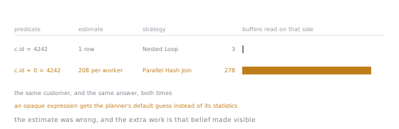
Read the row left to right and the causation is in the order: the estimate is what changed first, the strategy followed from it, and the bar is what followed from the strategy. Nothing about the data, the answer, or the index moved between the two rows.

The bare plan for that scan reads rows=208 per worker, over 600 times the true count of one: an opaque expression gets the planner's default guess instead of a lookup in its statistics, the same failure lesson 37 named for a correlated pair of columns. Believing the small side is no longer tiny, the planner drops the loop for a Parallel Hash Join; the 278 buffers that side alone now takes, against the 3 the correct plan touched for the same customer, is that belief showing up as work. enable_hashjoin, enable_mergejoin and enable_nestloop exist for exactly this kind of investigation, not as a fix to leave set.

work_mem, and the spill that reads like a signature

work_mem, default 4MB here, bounds how much memory one hash or sort node may build before writing to disk, applied per node rather than per statement, proved rather than stated below. Lowering it to 64kB for the KE hash join above turns its one-batch Hash into this:

->  Hash (actual rows=8332.00 loops=3)
      Buckets: 4096  Batches: 4  Memory Usage: 114kB
      Buffers: shared hit=2502, temp written=60
      ->  Seq Scan on customers c (actual rows=8332.00 loops=3)
            Filter: (country = 'KE'::text)

with the join's own buffers gaining temp read=2764 written=2764. A batch is one full pass of the hash table and the probe input; more than one means the build side did not fit, so it was partitioned to temporary files and read back once per batch, exactly what those temp figures count. That combination, more than one batch plus nonzero temp read/written, is the spill's signature on any machine. The two honest fixes are more memory, raising work_mem for the session, or fewer rows: filtering to country = 'NL', one customer rather than 8332, keeps Batches: 1 and Memory Usage: 9kB at the same 64kB.

That binding is per node, easy to miss with only one hash to watch. A three-table join, orders to customers to countries filtered to one region, has two, and at the same 64kB one spills while the other does not: the customers-side Hash, from 8332 rows, reads Buckets: 4096 Batches: 8 Memory Usage: 73kB; the countries-side Hash, from one row, reads Buckets: 1024 Batches: 1 Memory Usage: 9kB. One session, two budgets spent independently.

Parallel plans, named

Every plan above has printed a Gather without explaining it. Its sub-plan runs once per launched worker plus once in the leader, each contributing a partial result Gather combines into one stream. Workers Planned is what the plan asked for, capped at max_parallel_workers_per_gather, 2 here; Workers Launched is what it got, differing when the shared pool of background workers has fewer to hand over. Every Gather above launched exactly what it planned, so seeing them differ needs starving that pool on purpose: with max_parallel_workers lowered to 1, a parallel scan over amount > 400 plans for two workers and gets one:

Finalize Aggregate (actual rows=1.00 loops=1)
  ->  Gather (actual rows=2.00 loops=1)
        Workers Planned: 2
        Workers Launched: 1
        Buffers: shared hit=7608
        ->  Partial Aggregate (actual rows=1.00 loops=2)
              ->  Parallel Seq Scan on orders (actual rows=106032.00 loops=2)
                    Filter: (amount > '400'::numeric)
                    Rows Removed by Filter: 418926

Workers Launched: 1 against Workers Planned: 2 is no sign of anything broken; the count returned is still right, with the leader and one worker sharing what the plan expected two to share. The per-worker lines in the merge join above, Worker 0 and Worker 1 each with their own Sort Method, are the same idea one level down: a skewed join can leave one worker doing far more than another.

Join order, briefly

The planner also chooses which table meets which first, searching every order a limit allows and pricing each, the same principle as choosing between strategies. join_collapse_limit, 8 here, bounds how many FROM items an explicit JOIN chain may still be reordered among before the search takes them as written; from_collapse_limit, also 8, does the same for a folded subquery. Below the limit the search tries every order; above it, the planner switches to a cheaper heuristic instead. Written as orders JOIN customers JOIN countries, filtered to one region, the printed plan reorders it:

Hash Join (actual rows=27773.33 loops=3)
  Hash Cond: (o.customer_id = c.id)
  ->  Parallel Seq Scan on orders o (actual rows=349972.00 loops=3)
  ->  Hash (actual rows=8332.00 loops=3)
        ->  Hash Join (actual rows=8332.00 loops=3)
              Hash Cond: (c.country = n.code)
              ->  Seq Scan on customers c (actual rows=100000.00 loops=3)
              ->  Hash (actual rows=1.00 loops=3)
                    ->  Seq Scan on countries n (actual rows=1.00 loops=3)
                          Filter: (region = 'Africa'::text)

countries, filtered first to one row, and customers join at the bottom, before orders, the largest table and the last one named, is touched at all: the written order put orders first and countries last, and the executed order is the opposite, since pairing the two small sides first costs less than starting from the million-row table.

When the strategy looks wrong

A join with an expensive-looking strategy is usually a join handed a wrong estimate, lesson 37's material: check the estimated rows= on each side against what EXPLAIN (ANALYZE) returned, since the section above showed one wrong estimate flips a nested loop into a hash join with the data unchanged. Only once the estimate is confirmed right and the strategy still looks wrong is it worth reshaping the query: an index from lesson 38, a narrower filter, fewer columns read. Leaving an enable_* switch off past the investigation is not that reshaping: it removes a whole class of plan from every query on the connection, and a plan that looks better with one disabled may only look that way because its real best option was removed.

Practice

1. ▢ Predict whether forcing a nested loop onto the KE join, by turning enable_hashjoin and enable_mergejoin off, costs more or fewer buffers than the default hash join, then check.

2. ▢ The KE hash join's Hash node reads Buckets: 16384 Batches: 1 Memory Usage: 454kB at the default work_mem of 4MB. Predict those three figures at work_mem = '16MB', then check.

3. ▢ At work_mem = '64kB', the KE hash join spills to four batches. Predict the same setting's effect on a hash join filtered to country = 'NL', one customer rather than 8332, then check.

4. ▢ max_parallel_workers is lowered to 0 rather than 1, on the same amount > 400 query. Predict Workers Launched, and whether the count returned is still right.

5. ▢ join_collapse_limit is set to 1, on the three-table query from the join order section. Predict whether the printed order still reorders countries ahead of orders, then check.

6. ▢ The good-estimate and bad-estimate plans for customers.id = 4242 choose different strategies. Predict whether either can return a different count of matching rows because of that choice.

Real-world reps

• [ ] Find a join in your own workload and name which of the three strategies its plan uses.
• [ ] Run EXPLAIN (ANALYZE) on a join of your own, once as it is and once with the other two strategies switched off via enable_*, compare buffer counts, then reset every setting touched.
• [ ] Tomorrow: find a join or filter column wrapped in an expression, and check whether removing the wrapper changes the planner's row estimate the way id + 0 did here.

Going further

• 19.7.1. Planner Method Configuration: the enable_* switches used to force each strategy
• 14.3. Controlling the Planner with Explicit JOIN Clauses: join_collapse_limit and from_collapse_limit
• 19.4.1. Memory: work_mem and its neighbours
• 15.3. Parallel Plans: Gather, Workers Planned and Workers Launched
• Performance: the stage 6 reference sheet
• Resources

Not landing? Reread the primary source at the top, since this lesson compresses it and compression is where understanding leaks. Check the glossary for any term that felt slippery.

If the lesson itself is unclear rather than the material, that is a defect: open an issue.