Performance
Lookup sheet for stage 6. The question it exists to answer: which plan-derived count proves this query's shape, and which scan, join or index decision explains it?
Which numbers to trust
EXPLAIN (ANALYZE) prints two families of number, and only one survives a rerun on different hardware. Five runs of select count(*) from orders where customer_id = 4242 with no index gave execution times spread by about eight percent fastest to slowest, while Buffers: shared hit=7608 came back identical every time. A timing is a fact about the machine that produced it at that moment; a plan-derived count is a fact about the work done, reproducible on any copy of the same data.
| Reports | Reproducible? | Why |
|---|---|---|
rows, loops | Yes | Counted from the rows produced, not timed |
Buffers: shared hit/read | Yes | Pages touched; the total is stable even though the hit/read split varies with the cache |
Rows Removed by Filter | Yes | Counted |
Heap Fetches | Yes | Counted visits to the heap from an index-only scan |
Index Searches | Yes | Counted restarts of a B-tree probe |
Buckets / Batches / Memory Usage | Yes | Sizes chosen and reported, not durations |
Sort Method and its Disk/Memory figure | Yes | Which algorithm ran and how much space it used |
cost=.. (estimate) | No | Arbitrary planner units for comparing plans of the same query, not a promise about anything measurable |
Execution Time, Planning Time, any timing | No | Depends on the machine and its state at that instant |
The EXPLAIN options, and what release 18 changed
| Option | Adds or removes |
|---|---|
ANALYZE | Runs the statement for real, adding actual rows, loops and buffer counts; on a write, the write happens, so wrap it in BEGIN; ...; ROLLBACK; |
BUFFERS | Adds the Buffers lines; automatic under ANALYZE on release 18, so it is now only needed to add them to a bare EXPLAIN |
COSTS OFF | Removes cost=.. and estimated rows=, once the estimate has been compared against the actual |
TIMING OFF | Drops per-node timings, keeping row and buffer counts |
SUMMARY OFF | Drops Planning Time and Execution Time; Planning: Buffers, a count, still prints |
VERBOSE | Adds each node's output columns and schema-qualifies table names |
FORMAT JSON | Renders the same tree as structured data instead of indented text |
This stage's habit for a plan meant to be read is EXPLAIN (ANALYZE, COSTS OFF, TIMING OFF, SUMMARY OFF). Release 18 changed EXPLAIN's output in four places a reader comparing against older writing will notice: BUFFERS is automatic under ANALYZE; an index scan reports Index Searches; a per-loop average row count prints fractionally instead of rounding; and more node types report memory and disk figures once limited to a sort or a hash. See Lesson 35.
The plan nodes of this stage
| Node | What it does | The tell |
|---|---|---|
Seq Scan (Parallel Seq Scan) | Reads every page in physical order, split across workers under Gather | Rows Removed by Filter against rows: near-total discard is why it looks expensive |
Index Scan | Walks a B-tree to matching entries, visits the heap once per match | Buffers against rows: far more than one per match means scattered heap visits |
Index Only Scan | Walks the tree and answers from the leaf entries alone | Heap Fetches: 0 means the table was never opened |
Bitmap Heap Scan (over Bitmap Index Scan) | Collects matches first, then visits their heap pages once each, in order | Heap Blocks: exact=: fewer blocks than matching rows is the payoff |
Hash Join | Builds a hash table from the smaller side, probes it once with the larger | Batches: 1 fit work_mem; more means it spilled |
Merge Join | Sorts both sides by the join key and walks them together | The two Sort Method lines: in-memory against external merge on disk |
Nested Loop | Probes the inner side once per outer row, the literal filtered cross-product | Whether the inner side is Materialized or indexed; suspect a large, unindexed one |
Sort | Orders rows for a merge join, ORDER BY or GROUP BY | Sort Method: top-N heapsort/quicksort in memory against external merge spilled |
Gather (Gather Merge) | Collects each launched worker's partial result into one stream | Workers Launched against Workers Planned: fewer is not a fault |
Limit | Stops the input once enough rows exist | The child's rows: small means the bounded-scan bet paid off |
Aggregate (Partial/Finalize Aggregate) | Folds rows to one value or one per group, per worker first when parallel | rows on the node below: only as cheap as what it was handed |
The scan decision
The planner prices every candidate scan against random_page_cost (default 4) and seq_page_cost (default 1): a page read out of physical order costs four times one read in order.
| Scan kind | Wins when |
|---|---|
| Sequential (or parallel) | The predicate keeps a large share of the table, since seq_page_cost is paid once per page regardless of matches |
| Index scan | Selective enough that the walk plus a few random_page_cost heap visits beats reading every page, as customer_id = 4242 does at seven rows of 1,049,916 |
| Parallel index (only) scan | The same index still wins but the row count is large enough to split across workers, as customer_id < 33334, a third of the table |
| Index-only scan | An index scan would win, and every needed column already sits in the index, removing the heap visit |
| Bitmap heap scan | Too many matches for per-row heap visits to stay cheap, too few for a sequential scan to win; amount between 200 and 220, four percent of the table |
Raising random_page_cost or lowering seq_page_cost moves every crossover toward the sequential scan; the reverse moves them toward the index. See Lesson 36.
The index decisions
| Decision | What it means |
|---|---|
| Leftmost-prefix rule | An index on (a, b, c) serves a filter on a, on a and b, or on all three; b or c alone gets nothing, since only the leading column can start a walk (see below) |
| Multicolumn | Serves the query shapes sharing a leading column; (customer_id, amount) answers customer_id alone or with amount, and can remove a Sort on the trailing column too |
INCLUDE | Rides a column in the leaf pages for reading only, not searching; turns an Index Scan into an Index Only Scan, but a filter or ORDER BY on it still falls back to a scan or a Sort |
| Partial | Restricted by a WHERE on CREATE INDEX, staying small and serving only a query whose predicate implies the index's; a query outside that predicate cannot use it |
| Expression | Indexes a function's output, lower(email) rather than email, so a query wrapping the column the same way can match it; the plain column index cannot |
| Skip scan | New in release 18; reaches a non-leading column when the leading one has few distinct values, restarting once per value, seen as Index Searches above one for a single row; does nothing for a high-cardinality leading column |
| Refuse an index when | Not selective enough, so a sequential scan already wins; an existing index already serves it as a leftmost prefix; or the write cost, one more structure every INSERT/UPDATE/DELETE maintains, outweighs the read it buys |
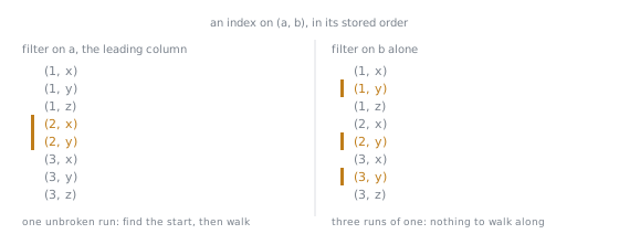
The leftmost-prefix rule is a fact about storage order, shown here on two columns rather than three. Sorting by a first puts every row sharing an a next to every other, so a filter on it is one run: find the start, then walk until the value changes. Sorting by a first also scatters the rows sharing a b, so a filter on b alone has no run to find and the walk never starts. The same reasoning is why the rule extends to c, and why (a, b) and (b, a) are different indexes.
See Lesson 38.
Statistics
pg_stats holds what one ANALYZE sampled, and every rows= estimate in every plan is arithmetic on these stored numbers, done before a single row of the query is read.
| Column | Estimates |
|---|---|
n_distinct | Distinct value count: positive is an absolute headcount (usually an underestimate on a sample), negative is minus the ratio of distinct values to rows, so -1 means one per row |
most_common_vals / most_common_freqs | Values worth pricing individually, and how common each is; empty when nothing stands out |
histogram_bounds | The range split into roughly equal-frequency buckets, priced by BETWEEN or < once no most_common_vals entry covers it |
correlation | How closely disk order matches sorted order, -1 to 1; near 1 (or -1) means neighbouring rows sit together, near 0 means scattered |
These are a sample, not a census, so the values differ between ANALYZE runs on unchanged data, unlike a buffer count: one run read customer_id's n_distinct at 78843 against a true 100000, and another run reads a different number. default_statistics_target, 100 by default, sets the sample size and can be raised per column with ALTER TABLE ... ALTER COLUMN ... SET STATISTICS. ANALYZE refreshes all of it; autovacuum queues its own run once more than autovacuum_analyze_threshold (50) plus autovacuum_analyze_scale_factor (0.1) times the row count has changed, about 105042 rows on orders. CREATE STATISTICS ... (dependencies, ndistinct) fixes the one thing a per-column sample cannot see, two columns moving together priced as independent, but only for an equality condition or a column compared to an expression; nothing for a range or a LIKE, so the same misestimate returns the moment = becomes BETWEEN. See Lesson 37.
Join strategies
| Strategy | Chosen when | work_mem signature of a spill |
|---|---|---|
| Hash join | One side is small enough to build a hash table from in one pass; the default for most joins here | Batches above 1 with temp read/written: the build side did not fit work_mem (default 4MB) and was partitioned to disk |
| Merge join | Both sides are already sorted by the join key, or forced by disabling the other two; pays a Sort up front otherwise | Sort Method: external merge with a Disk figure on the larger side; the smaller side often stays an in-memory quicksort |
| Nested loop | One side is confidently tiny, typically a primary-key lookup; the inner side is Materialized so it is read once and replayed | None of its own; the risk is a wrong estimate making a large side look tiny |
work_mem binds per node, not per statement: a three-table join can have two Hash nodes at the same setting, one spilling and the other not, by how many rows each side builds from. The enable_hashjoin, enable_mergejoin and enable_nestloop switches force a strategy for investigation only; reset them at once, since each removes a whole class of plan from every later query on the connection. See Lesson 39.
Pagination and counting
OFFSET walks the sort order from the start and discards every row before the one it returns; a keyset condition on the last row already seen starts exactly where the previous page ended. On orders ordered by id descending: the first page reads rows=20.00 at 4 buffers; the same page at OFFSET 500000 reads rows=500020.00 at 4993 buffers for the same twenty rows; the keyset rewrite, WHERE id < ..., is back to rows=20.00 at 7 buffers regardless of depth. OFFSET's cost grows with the offset; keyset's does not. A keyset condition on a non-unique sort column needs the same tiebreaker in WHERE as ORDER BY, compared as a row constructor, (customer_id, id) > (9, 1008), or it silently skips rows sharing the last-seen leading value.
Three honest answers to "how many rows match":
| Method | Cost | What it is for |
|---|---|---|
count(*), exact | Reads every matching page, the whole table for an unfiltered count | The true number, when worth a full pass |
reltuples from pg_class | Free, a stored estimate | Maintained by ANALYZE and autovacuum, so it drifts between refreshes; good for "roughly how many" |
Bounded, ... LIMIT n wrapped in count(*) | Stops once n matches are found | "More than n" cheaply; the true number when fewer than n match |
See Lesson 40.
When it is not the query
A query can be perfectly planned and still be slow because the table underneath it, or the client above it, is the real problem. A purpose-built 200,000-row table at 27 MB, fully updated once, grows to 54 MB with every row dead beside its new version. A plain VACUUM marks the dead space reusable, not returned: dead_tuple_percent falls to 0.0 and free_percent rises, but the file stays 54 MB. VACUUM FULL shrinks it back to 27 MB, at the cost of an ACCESS EXCLUSIVE lock for the rewrite. Two views answer "is this the table" with nothing to install: pg_stat_user_tables (n_live_tup, n_dead_tup, last_autovacuum) and pg_stat_all_indexes (idx_scan, for finding an index that costs every write and pays nothing back). pgstattuple needs only CREATE EXTENSION pgstattuple, turning a guess about bloat into a percentage. pg_stat_statements cannot be demonstrated without a server restart: it installs, but querying its view fails at once with ERROR: pg_stat_statements must be loaded via "shared_preload_libraries", SQLSTATE 55000, since the module must load at server start. Beyond the table, three causes never reach the server as a plan worth reading: the same statement run once per row from a client-side loop, a connection opened per request, and a full result set fetched when only a page was shown. See Lesson 41.
Diagnostics and settings
| Setting | Default, verified | Decides |
|---|---|---|
shared_buffers | 128MB | How much cache a Buffers: shared hit can be served from before falling to read |
work_mem | 4MB | How much memory one sort or hash node builds before spilling to disk, per node |
max_parallel_workers_per_gather | 2 | The ceiling on Workers Planned under one Gather |
max_parallel_workers | 8 | The server-wide pool Workers Launched draws from |
random_page_cost | 4 | The charge for an out-of-order page read, against seq_page_cost's 1; raising it favours sequential and index-only scans |
seq_page_cost | 1 | The charge for a page read in physical order |
track_io_timing | off | Whether a plan can report per-buffer timing; off here, so this stage never quotes one |
default_statistics_target | 100 | The sample size and most_common_vals/histogram length ANALYZE keeps per column |
autovacuum_analyze_threshold | 50 | The flat row-change count added to the scale factor before an automatic ANALYZE queues |
autovacuum_analyze_scale_factor | 0.1 | The fraction of a table's rows that must also change first |
join_collapse_limit | 8 | How many explicitly JOINed tables the planner still searches every order among |
from_collapse_limit | 8 | The same bound for a subquery folded into its parent |